mex_ports

A geospatial dataset of Mexican ports

Latest version:

By: Emma Zgonena, Renato Molina & Juan Carlos Villaseñor-Derbez

Cite all versions as: as: Zgonena et al., 2025. A geospatial dataset of Mexican ports. DOI: 10.5281/zenodo.15778574

Overview

This repository contains data and code to build a geospatial dataset of the major ports of Mexico, some of which are included in CONAPESCA’s landing data. It is intended to interface with other data in mex_fisheries, such as vessel- and port-level landings information.

How the data are built

1) Extract port information and location

The final data, mex_ports, is a culmination of information from the files mexian_ports.csv and mex_large_scale_landing_ports.csv that are correlated through mex_ports_dictionary.csv.

The information originates from the pdf titled catastro.pdf, which contains information on Mexican ports from the Mexican Secretaria de Comunicaciones y Transportes and the Departamento de Catastro, Instalaciones y Recintos. K+The following key variables were manually extracted from the PDF to create mexian_ports.csv:

The inputs for port_id are labeled as ‘Clv. del puerto’ in catastro.pdf
The inputs for municipality_code (renamed municipality_id in final mex_ports cleaned data) and municipality_name are found labeled together under ‘Municipio’ in catastro.pdf
The inputs for port_name are labeled as Nombre del Puerto in catastro.pdf
The inputs for longitude and latitude are labeled as Longitud and Latutid respectively in catastro.pdf

Note: 155 individual ports were identified in mexican_ports.csv, 4 of which are on lakes and therefore are not coastline ports.

2) Identify ports with recorded fisheries landings

The information in mex_large_scale_landing_ports.csv is from Mexico’s fisheries production data. Code showing the extraction is included in 01_get_large_scale_ports.R. The data do not include port_id, and instead use CONAPESCA’s system of unique identifiers (mex_ports_id). We manually built a dictionary (mex_ports_dictionary.csv) that allowed us to link port_ids to landinge_site_keys.

Note: 51 of the total ports in mexican_ports.csv can be matched to ports in mex_large_scale_landing_ports.csv

3) Combine data

The final data, mex_ports, was created using the script titled 03_combine_sources.R.

This script cleans and retains relevant columns from the dictionary, omitting lake ports (4) that are not relevant to the set. It then combines the objects through their corresponding port_id. Finally, the data is standardized in name and made further accessible through the addition of tabular and geospatial file versions.

Note: The final data set has 151 ports, of which 55 can be matched to CONAPESCA’s mex_ports_id

Metadata

Data files

The data are available in three formats:

mex_ports.gpkg: A geopackage in EPSG:4326. This is the recommended source because it is already a spatial object.
mex_ports.rds: Tabular format as an R object.
mex_ports.csv: Tabular format as a comma-separated values file.

Column specifications across all are the same

municipality_id or municipality_code: character. 5-digit code that acts as a unique identifier for each municipality.
municipality_name: character. Official name of municipality.
port_id: character. 5-digit code that acts as a unique identifier for each port.
port_name: character. Official name of port. Originally labeled under ‘Nombre del Puerto’.
landing_site_id: character. 3-digit alphanumeric string that acts as a unique identifier for a what CONAPESCA considers a landing site. Note that ports not matched to a landing site id will show NA in this column.
latitude: numeric. Latitude in decimal degrees for the location of the port.
longitude: numeric. Longitude in decimal degrees for the location of the port.

Using the data

Build a table of landing sites an d corodinates

#Load packages

library(tidyverse)
# Load the data using the csv file
mex_ports <- read_csv(
  file = "https://github.com/mex-fisheries/mex_ports/raw/refs/heads/main/data/clean/mex_ports.csv") # You can read the rds file using read_RDS(url("url/to/file.rds"))
#> Rows: 151 Columns: 7
#> ── Column specification ────────────────────────────────────────────────────────
#> Delimiter: ","
#> chr (5): municipality_id, municipality_name, port_id, port_name, landing_sit...
#> dbl (2): longitude, latitude
#> 
#> ℹ Use `spec()` to retrieve the full column specification for this data.
#> ℹ Specify the column types or set `show_col_types = FALSE` to quiet this message.

# A quick glimpse at the data
glimpse(mex_ports)
#> Rows: 151
#> Columns: 7
#> $ municipality_id   <chr> "02005", "02001", "02001", "02001", "02001", "02001"…
#> $ municipality_name <chr> "PLAYAS DE ROSARITO", "ENSENADA", "ENSENADA", "ENSEN…
#> $ port_id           <chr> "02001", "02002", "02003", "02004", "02005", "02006"…
#> $ port_name         <chr> "ROSARITO", "LA MISION", "El SAUZAL", "MARINA CORAL"…
#> $ landing_site_id   <chr> NA, NA, "02A", NA, "02B", NA, NA, NA, "02C", "02D", …
#> $ longitude         <dbl> -117.0731, -116.8801, -116.7043, -116.6612, -116.625…
#> $ latitude          <dbl> 32.3692, 32.0550, 31.8944, 31.8622, 31.8522, 31.5176…

# Let's get all ports that can be matched to landing site from CONAPESCA's data
mex_ports |> 
  filter(!is.na(landing_site_id)) |> 
  select(port_name, landing_site_id, longitude, latitude)
#> # A tibble: 50 × 4
#>    port_name       landing_site_id longitude latitude
#>    <chr>           <chr>               <dbl>    <dbl>
#>  1 El SAUZAL       02A                 -117.     31.9
#>  2 ENSENADA        02B                 -117.     31.9
#>  3 ISLA CEDROS     02C                 -115.     28.1
#>  4 SAN FELLIPE     02D                 -115.     31.0
#>  5 GURRERO NEGRO   03L                 -114.     27.9
#>  6 A. LOPEZ MATEOS 03D                 -112.     25.2
#>  7 SAN CARLOS      03B                 -112.     24.8
#>  8 PUERTO ALCATRAZ 03C                 -112.     24.5
#>  9 CABO SAN LUCAS  03E                 -110.     22.9
#> 10 SANTA ROSALIA   03H                 -112.     27.3
#> # ℹ 40 more rows

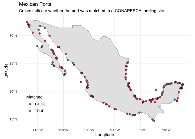
Build a map

The code below is used to build the figure at the top of this document.

# Load packages
library(rnaturalearth)
library(sf)
library(tidyverse)

# This time we read the geopackage
mex_ports_sf <- st_read("https://github.com/mex-fisheries/mex_ports/raw/refs/heads/main/data/clean/mex_ports.gpkg",
                        quiet = TRUE)

mex <- ne_countries(country = "Mexico")

ggplot(data = mex) +
  geom_sf() +
  geom_sf(data = mex_ports_sf,
          mapping = aes(fill = !is.na(landing_site_id)),
          color = "black",
          shape = 21,
          size = 2,
          alpha = 0.7) +
  theme_minimal() +
  theme(legend.position = "inside",
        legend.position.inside = c(0.1, 0.2)) +
  scale_fill_brewer(palette = "Set1") +
  labs(title = "Mexican Ports",
       subtitle = "Colors indicate whether the port was matched to a CONAPESCA landing site",
       x = "Longitude",
       y = "Latitude",
       fill = "Matched")

This site is open source. Improve this page.